Detecting Music BPM using Neural Networks

I have always wondered whether it would be possible to detect the tempo (or beats per minute, or BPM) of a piece of music using a neural network-based approach. After a small experiment a while back, I decided to make a more serious second attempt. Here’s how it went.

Approach

Initially I had to throw around a few ideas regarding the best way to represent the input audio, the BPM, and what would be an ideal neural network architecture.

Input data format

One of the first decisions to make here is what general form the network’s input should take. I don’t know a whole lot about the physics side of audio, or frequency data more generally, but I am familiar with Fourier analysis, and spectograms.

I figured a frequency spectogram would serve as an appropriate input to whatever network I was planning on training. These basically contain time on the x-axis, and frequency bins on the y-axis. The values (pixel colour) then indicate the intensity of the audio signal at each frequency and time step.

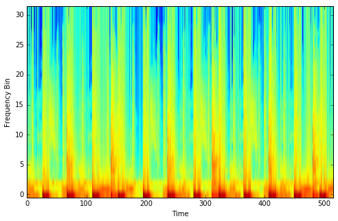
An example frequency spectogram from a few seconds of electronic music. Note the kick drum on each beat in the lowest frequency bin.

Output data format (to be predicted by the network)

I had a few different ideas here. First I thought I might try predicting the BPM directly. Then I decided I could save the network some trouble by having it try to predict the location of the beats in time. The BPM could then be inferred from this. I achieved this by constructing what I call a ‘pulse vector’ as follows:

• Say we had a two second audio clip. We might represent this by a vector of zeroes of length 200 - a resolution of 100 frames per second.

• Then say the tempo was 120 BPM, and the first beat was at the start of the clip. We could then create our target vector by setting (zero-indexed) elements [0, 50, 100, 150] of this vector to 1 (as 120 BPM implies 2 beats per second).

We can relatively easily infer BPM from this vector (though its resolution will determine how accurately). As a bonus, the network will also (hopefully) tell us where the beats are, in addition to just how often they occur. This might be useful, for instance if we wanted to synchronise two tracks together.

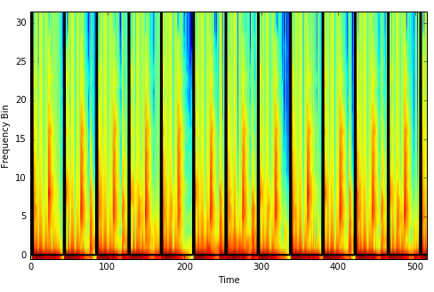
This image overlays the target output pulse vector (black) over the input frequency spectogram of a clip of audio.

Neural network architecture

My initial architecture involved just dense layers. I was working in Lasagne. I soon discovered the magic of Keras however, when looking for a way to apply the same dense layer to every time step. After switching to Keras, I also added a convolutional layer. So the current architecture is essentially a convolutional neural network. My intuition behind the inclusion and order of specific network layers is covered further below.

Creating the training data

The main training data was obtained from my Traktor collection. Traktor is a DJing program, which is quite capable of detecting the BPM of the tracks you give it, particularly for electronic music. I have not had Traktor installed for a while, but a lot of the mp3 files in my music collection still have the Traktor-detected BPM stored with the file.

I copied around 30 of these mp3’s to a folder, however later realised that they still needed a bit more auditing - files needed to start exactly on the first beat, and needed to not get out of time throughout the song under the assumed BPM. Therefore I opened each in Reaper (a digital audio workstation), chopped each song to start on exactly the first beat, ensured they didn’t go out of time, and then exported them to wav.

Going from mp3/wav files to training data is all performed by the mp3s_to_fft_features.py script.

~I then converted¹ these to wav and read them into Python (using wavio). I also read the BPM from each mp3 into Python (using id3reader).~

-> I now already already have the songs in wav format, and the BPMs were read from the filenames, which I manually entered.

The wav is then converted to a spectogram. This was achieved by:

1. Taking a sample of length fft_sample_length (default 768) every fft_step_size (default 512) samples
2. Performing a fast fourier transform (FFT) on each of these samples

The target pulse vector matching the wav’s BPM is then created using the function get_target_vector.

Then random subsets of length desired_X_time_dim are taken in pairs from both the spectogram and target pulse vector. By this, we generate lots of training inputs and outputs that are a more manageable length from just the one set of training inputs. Each sample represents about 6 seconds of audio, with different offsets for where the beats are placed (so our model has to predict where the beats are, as well as how often they occur).

For each ~6 second sample, we now have a 512x32 matrix as training input - 512 time frames and 32 frequency bins (the number of frequency bins can be reduced by increasing the downsample argument) - and a 512x1 pulse vector as training output.

In the latest version of the model, I have 18 songs to sample from. I create a training set by sampling from the first 13 songs, and validation and test sets by sampling from the last 5 songs. The training set contained 28800 samples.

Specifying and training the neural network

Network architecture - overview

As described above, I decided to go with a convolutional neural network architecture. It looked something like this:

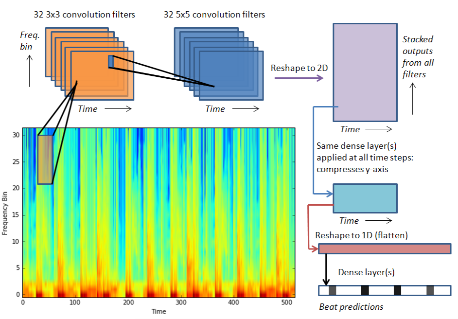
An overview of the neural network architecture.

In words, the diagram/architecture can be described as follows:

• The input spectogram is passed through two sequential convolutional layers

• The output is then reshaped into a ‘time by other’ representation

• Keras’ TimeDistributed Dense layers are then used (in these layers, each time step is passed through the same dense layer; this substantially reduces the number of parameters needed to be estimated)

• Finally, the output is reduced to one dimension, and passed through some additional desnse layers before producing the output

Network architecture - details

The below code snippets give specific details as to the network architecture and its implementation in Keras.

First, we have two convolution layers:

model = Sequential()

model.add(Convolution2D(num_filters, 3, 3, border_mode='same', 
                        input_shape=(1, input_time_dim, input_freq_dim)))
model.add(Activation('relu'))

model.add(MaxPooling2D(pool_size=(1,2)))

model.add(Convolution2D(num_filters, 5, 5, border_mode='same'))
model.add(Activation('relu'))

I limited the amount of max-pooling. Max-pooling over the first dimension would reduce the time granularity, which I feel is important in our case, and in the second dimension we don’t have much granularity as it is (just the 32 frequency bins). Hence I only performed max pooling over the frequency dimension, and only once. I am still experimenting with the convolutional layers’ setup, but the current configuartion seems to produce decent results.

I then reshape the output of the convolution filters so that we again have a ‘time by other stuff’ representation. This allows us to add some TimeDistributed layers. We have a matrix input of something like 512x1024 here, with the 1024 representing the outputs of all the convolutions. The TimeDistributed layers allow us to go down to something like 512x256, but with only one (1024x256) weight matrix. This dense layer is then used at all time steps. In other words, these layers densely connect the outputs at each time step to the inputs in the corresponding time steps of the following layer. The overall benefit of this is that far fewer parameters need to be learned.

The intuition behind this is that if we have a 1024-length vector representing each time step, then we can probably learn a useful representation at a lower dimension of that time step, which will get us to a matrix size that will actually fit in memory when we try to add some dense layers afterwards.

model.add(Reshape((input_time_dim, input_freq_dim * num_filters)))

model.add(TimeDistributed(Dense(256)))
model.add(Activation('relu'))
model.add(TimeDistributed(Dense(8)))
model.add(Activation('relu'))

Finally, we flatten everything and add a few dense layers. These simultaneously take into account both the time and frequency dimensions. This should be important, as the model can try to incorporate things like the fact that beats should be evenly spaced over time.

model.add(Flatten())

for w in dense_widths:
    model.add(Dense(w))
    model.add(Activation('relu'))
    model.add(Dropout(drop_hid))
model.add(Dense(output_length))
model.add(Activation('relu'))

Results

Usually the model got to a point where validation error stopped reducing after 9 or so epochs.

With the current configuration, the model appears to be able to detect beats in the music to some extent. Note that I’ve actually switched to inputs and outputs of length 160 (in the time dimension), though I was able to achieve similar results on the original 512-length data.

This first plot shows typical performance on audio clips within the training set:

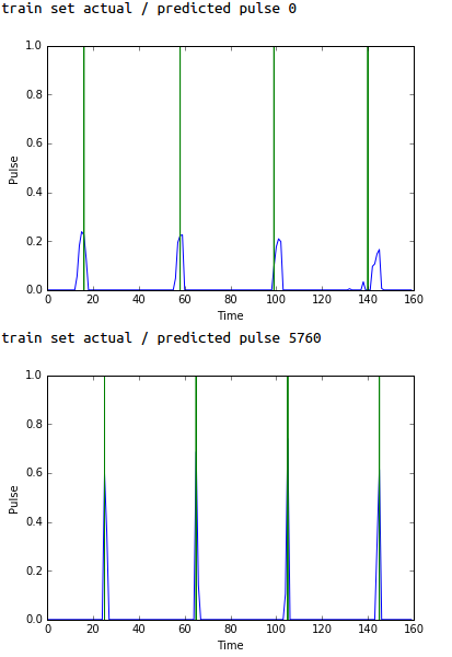
Predicted (blue) vs actual (green) pulses - typical performance over the training set.

Performance is not as good when trying to predict pulse vectors derived from songs that were not in the training data. That said, on some songs the network still gets it (nearly) right. It also often gets the frequency of the beats correct, even though those beats are not in the correct position:

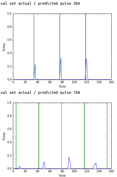
Predicted (blue) vs actual (green) pulses - typical performance over the validation set.

If we plot these predictions/actuals over the input training data, we can compare our own intuition to that of the neural network:

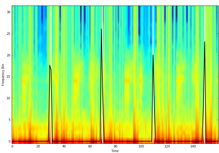
Predicted (black) vs actual (white) pulses plotted over spectogram - typical performance over the training set.

Take this one validation set example. I would find it hard to tell where the beats are by looking at this image, but the neural net manages to figure it out at least semi-accurately.

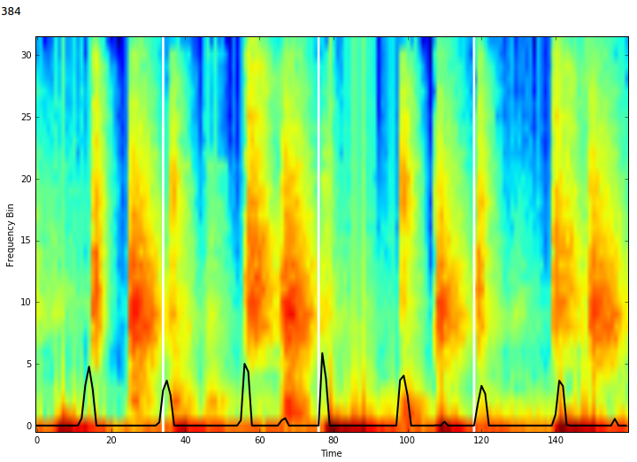
Predicted (black) vs actual (white) pulses plotted over spectogram - typical performance over the validation set.

Next steps

This is still a work in progress, but I think the results show far have shown that this approach has potential. From here I’ll be looking to:

• Use far more training data - I think many more songs are needed for the neural network to learn the general patterns that indicate beats in music

• Read up on convolutional architectures to better understand what might work best for this particular situation

• An approach I’ve been thinking might work better: adjust the network architecture to do ‘beat detection’ on shorter chunks of audio, then combine the output of this over a longer duration. This longer output can then serve as the input to a neural network that ‘cleans up’ the beat predictions by using the context of the longer duration

I still need to clean up the code a bit, but you can get a feel for it here.

Random other thoughts

• I first thought of approaching this problem using a long-short term memory (LSTM) network. The audio signal would be fed in frame-by-frame as a frequency spectogram, and then at each step the network would output whether or not that time step represents the start of a beat. This is still an appealing prospect, however I decided to try a network architecture that I was more familiar with

• I tried a few different methods for producing audio training data for the network. For the proof-of-concept phase, I created a bunch of wav’s with just sine tones at varying pitches, decaying quickly and played only on the beat, at various BPM’s. It was quite easy to get the network to learn to recognise the BPM from these. A step up from this was taking various tempo-synced break beats, and saving them down at different tempos. These actually proved difficult to learn from - just as hard as real audio files

• It might be also interesting to try working with the raw wav data as the input

Footnotes

1: In the code, the function convert_an_mp3_to_wav(mp3_path, wav_path) tells Linux to use mpg123 to convert the input mp3_path to the output wav_path. If you are on Linux, you may need to install mpg123. If you are using a different operating system, you may need to replace this with your own function that converts the input mp3 to the output wav.