Detecting Music BPM using Neural Networks - Update

This post is a brief update to my previous post about using a neural network to detect the beats per minute (BPM) in short sections of audio.

This post is also accompanied by a new, more complete and commented version of the code. I have also decided to upload the training and validation data I used.¹

If you just want to see or run the code yourself, then feel free to skip ahead.

Key changes

The key differences between this and the last version are:

• I now use the raw audio (downsampled to 11kHz) as the input to the neural network, rather than a spectogram

• The raw audio vector is reshaped into a matrix of audio chunks, which are all processed in the same way. By default, 4 seconds of audio is represented by a 44100-length vector, which is reshaped into a matrix of size 441x100 (441 ‘timesteps’ with 100 ‘features’)

• This input matrix is then fed into a neural network architecture that is much simpler: just a Convolution1D layer followed by max pooling

• Training samples are now extracted randomly during training from the full-length audio files. This is achieved through the DataGen class. This means a much larger number of training samples can be synthesised without using additional memory

The Keras neural network specification now looks like this:

# Specify and compile the neural network model
max_pool = 4
model = Sequential()
model.add(Convolution1D(4 * max_pool, 3, border_mode='same', 
                        input_shape=(gen_train.num_chunks, 
                                     gen_train.num_features)))
if max_pool > 1:
    model.add(Reshape((1764 * max_pool, 1)))
    model.add(MaxPooling1D(pool_length=max_pool))
model.add(Activation('relu'))
model.add(Flatten())
model.summary()
model.compile(loss='mse', optimizer=Adam())

Let’s break this network topology down. We have:

1. An input of size (4 seconds * 44100 hz / 4 (downsampling rate)) = 44100 length vector (actually this is reshaped to 441x100 prior to input)
2. This is fed into a Convolution1D layer, with 4 * max_pool (=4 by default) filters, and a 1D convolution filter size of 3
3. A Reshape() layer just flattens the output of all these filters into one long vector
4. Max pooling takes the max of every 4 numbers in this vector
5. Then this goes through a ReLU activation

Figuring out what Keras’ Convolution1D layer is actually doing

The only tricky thing here is the Convolution1D layer. It took me a while to figure out exactly what this is doing, and I couldn’t find it explained that clearly anywhere else on the web, so I’ll try to explain it here:

• The Convolution1D layer takes an input matrix of shape Time Steps x Features

• It then reduces this to something of shape Time Steps x 1. So essentially it reduces all of the features to just a single number

• However, it does this for each filter, so if we have 16 filters, we end up with an output matrix of size Time Steps x 16

• But, assuming we have just one filter, it convolves that 1D filter over the features. So if you imagine we have time steps on the horizontal axis, and features on the vertical axis, at every time step, it passes the same 1D convolution filter over the vertical axis

• Then, a dense layer is used to go from a matrix of size Time Steps x Features to a matrix of size Time Steps x 1. So basically a weighted combination of the post-convolution features is taken at every time step. The same weights are used for all time steps

• These last two steps are repeated for each filter, so actually we end up with an output matrix of size Features x Num. Filters

Results and performance

Training set performance

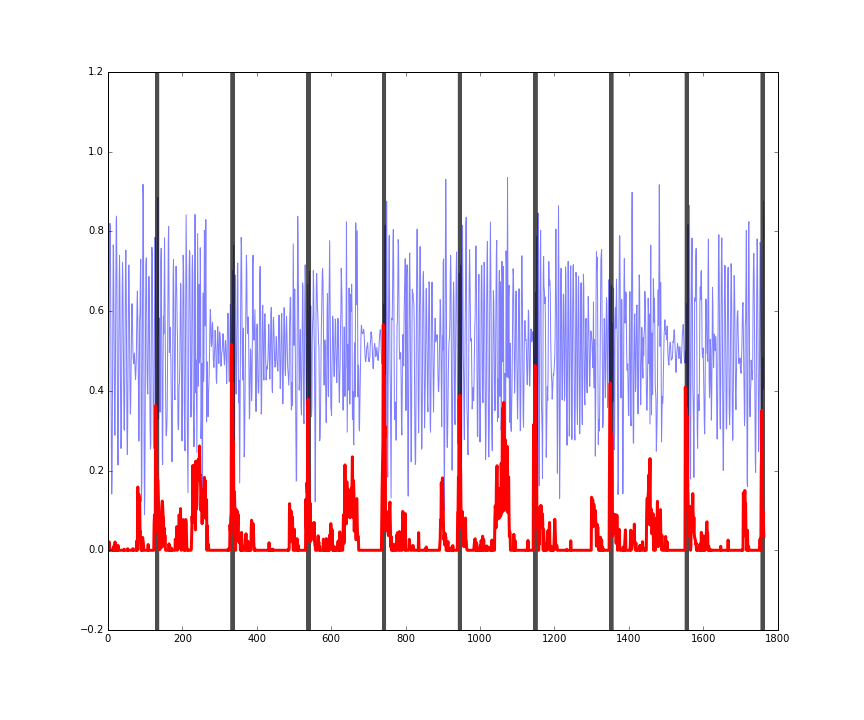
Here is the performance on three random four second sections of songs in the training set. You can see the audio in blue, the actual beats in black, and the predicted beats in red.

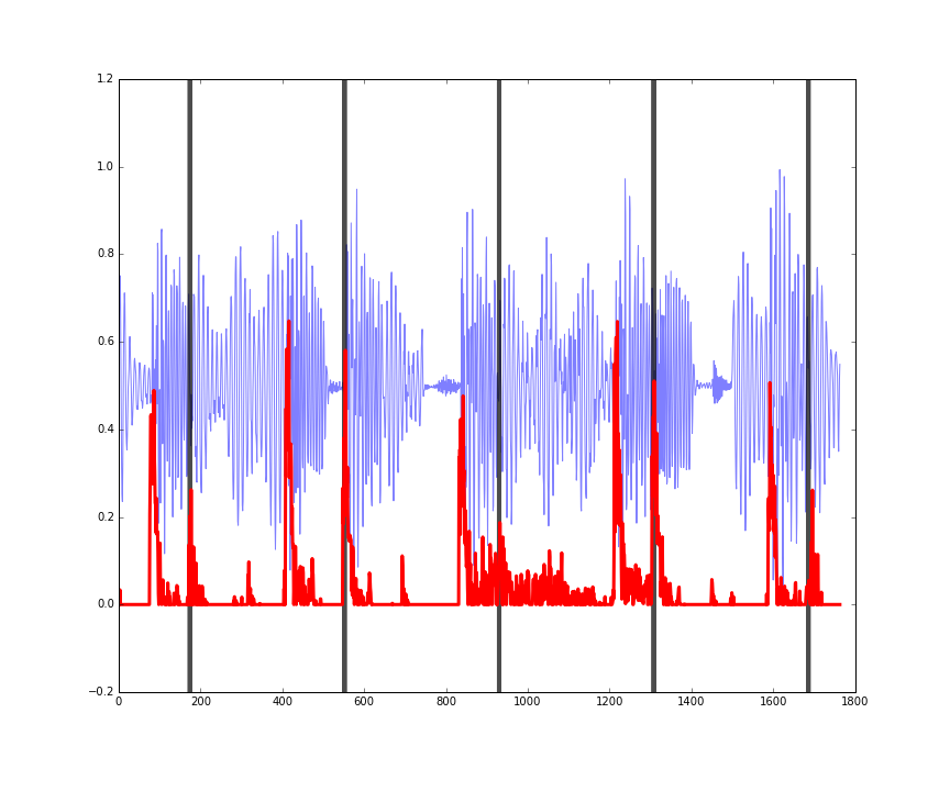
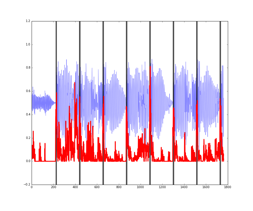
Figures: performance on some random four second clips of audio from the training set.

The predictions (red) might seem a bit noisy, but they’re still doing a pretty good job of picking up the onset of drum hits in the music.

The last figure shows how this is working more as an onset detector, rather than predicting where the actual beats of the bar are. In other words, it is working more as a ‘drum hits detector’ rather than a ‘beats in a bar detector.’

This is still useful however, and in some circumstances desirable. We can’t really expect our program to detect where the beats are by looking at just four seconds of audio. However by applying this predictor to larger sections of audio, the autocorrelation function of the predicted onsets can be used to infer the BPM (I experimented with this, and found it to be quite an accurate way of detecting the BPM: it was usually within 1 or 2 BPM of the actual song BPM in about 90% of tracks).

Validation set performance

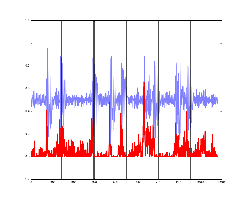
Another nice outcome is that performance on the validation data is pretty much the same as that on training data, meaning that the patterns the model has learned generalise well (at least to similar tracks, since I’ve only trained with electronic music):

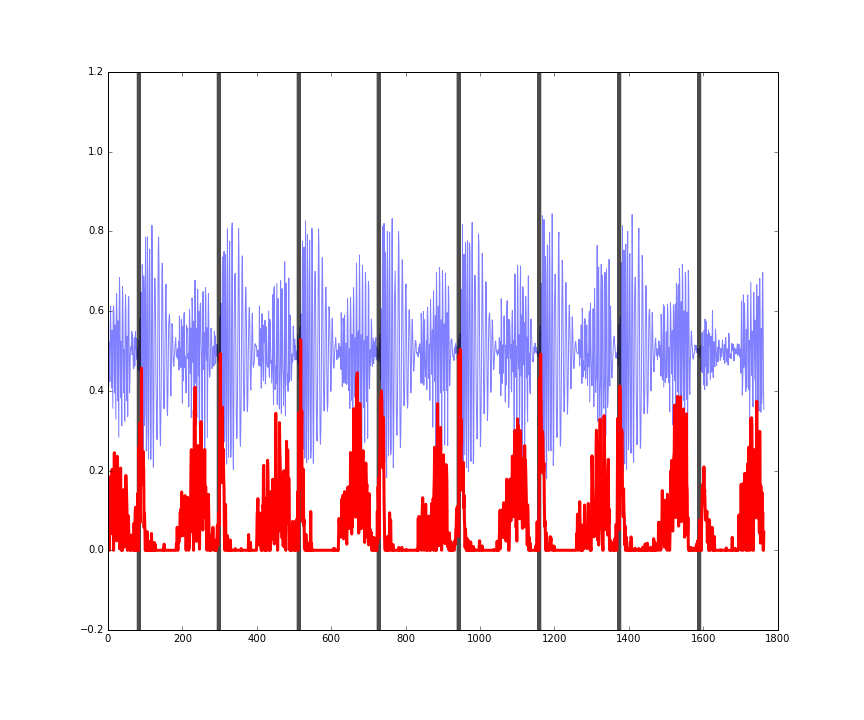
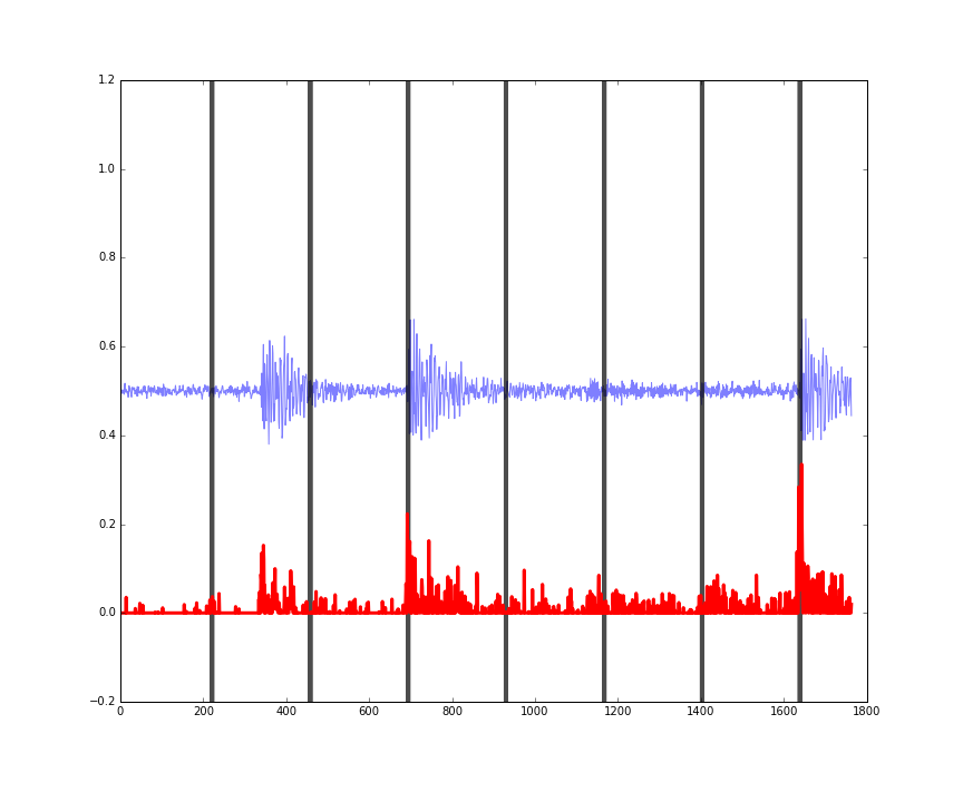Figures: performance on some random four second clips of audio from the validation set.

The last figure here also shows that the predictions are somewhat invariant to the amplitude (loudness) of the music being analysed.

How to run the code

To run the code yourself:

1. Clone the repo
2. Extract the training and validation data to the root of that repo
3. Run fit_nn.py to train the neural network and visualise the results
4. Alternatively or additionally, you could create your own training data by placing 44.1kHz .wavs in the wavs subdirectory, and then running wavs_to_features.py. These .wavs need to start exactly on the first beat, and have their true integer BPM as the first thing in the filename, followed by a space (see comments in code for further explanation).

Final thoughts

I played around with other, more complex network topologies, but found that this simple Convolution1D structure worked much better than anything else. Its simplicity also makes it very fast to train (at least on the quite old GPU in my laptop).

It is very curious that this network structure works so well. The output of each filter only has 441 timesteps, but it is clear that the predictions from the model are much more granular than this. It seems that certain filters are specialising in particular sections of each of the 441 time ‘chunks.’

In future it would be very interesting to drill down into the weights and see how this model is actually working. If anyone else wants to look into this then please do, and please share your findings!

Thanks for reading - would love to hear any thoughts!

Footnotes

1: I figure sharing 11kHz audio embedded in Python objects isn’t too bad a violation of copyright - if any of the material owners find this and disagree please feel free to get in contact with me and I will take it down.