Semi-Supervised Learning (and more): Kaggle Freesound Audio Tagging

An overview of semi-supervised learning and other techniques I applied to a recent Kaggle competition.

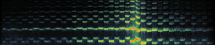
A spectrogram of of the audio clips in the FAT2019 competition

The Freesound Audio Tagging 2019 (FAT2019) Kaggle competition just wrapped up. I didn’t place too well (my submission was ranked around 144th out of 408 on the private leaderboard). But winning wasn’t exactly my focus. I tried some interesting things and would like to share what I did, plus provide some explanations and code so others might be able to benefit from my work.

This post starts with a brief overview of the competition itself. Then I work chronologically through the main ideas I tried, introducing some of the theory behind each. I also provide some code snippets illustrating each method.

The competition

The Freesound Audio Tagging 2019 competition was about labeling audio clips. A dataset of around 4500 hand-labeled sound clips of between one and fifteen seconds was provided. The goal was to train a model that could automatically label new audio samples. There were 80 possible labels, ranging from ‘acoustic guitar’ to ‘race car’ to ‘screaming’. Audio samples could be tagged with one or more labels. Here are a few examples:

Labels = [Accelerating_and_revving_and_vroom, Motorcycle]

Labels = [Fill_(with_liquid)]

Labels = [Cheering, Crowd]

My starting point - mhiro2’s public kernel

Like many other entrants, my starting point was a public kernel submitted by kaggler mhiro2. This kernel classified samples via a convolutional neural network (convnet) image classifier architecture. ‘Images’ of each audio clip were created by taking the log-mel spectrogram of the audio signal. 2-second subsets of the audio clips are randomly selected, and the model is then trained via a binary cross-entropy loss (as this is a multi-label classification task). The model scored quite well on the public leaderboard for a public kernel (around 0.610 if I remember correctly).

Skip connections

I was able to get a big boost in score (~0.610 –> ~0.639) through simply adding DenseNet-like skip connections to this kernel. I implemented skip connections by concatenating each network layer’s input with its output, prior to downsampling via average pooling.

What is it?

Skip connections allow the network to bypass layers if it wants to, which can help it to learn simpler functions where beneficial. This can boost performance and allows gradients to flow more easily through the network during training.

Implementation for FAT2019

The change is illustrated in my kernel fork and this code snippet:

def forward(self, input):
    x = self.conv1(input)
    x = self.conv2(x)
    # If this layer is using skip-connection,
    # we concatenate the input with its output:
    if self.skip:
        x = torch.cat([x, input], 1)
    x = F.avg_pool2d(x, 2)
    return x

Cosine annealing learning rate scheduling

Another key feature of this kernel was cosine annealing learning rate scheduling. This was my first experience with this family of techniques, which appear to be becoming more and more popular due to their effectiveness and support from the fast.ai community.

What is it?

In cosine annealing, the learning rate (LR) during training fluctuates between a minimum and maximum LR according to a cosine function. The LR is updated at the end of each epoch according to this function.

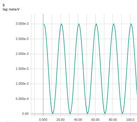
The learning rate (y-axis) used in training over epochs (x-axis) when cosine annealing is enabled

The ideas behind cosine annealing LR were introduced in this paper. Often, cosine annealing leads to two main benefits:

• Training is faster
• A better final network is found - despite being faster to train, often the final model obtained produces better test set results than under traditional stochastic gradient descent (SGD)

The main theory behind why cosine annealing (or SGD with restarts) leads to better results is well-explained in this blog post. In short, there are two purported modes of action:

1. The periods with a large learning rate allow the model to ‘jump’ out of bad local optima to better ones.
2. If a stable optimum is found that we do not jump out of when we return to a high learning rate, this optimum is likely more general and robust to shifts in the data distribution, and thus leads to better test performace.

Cosine LR annealing to be seems to be a really effective technique. I’m also curious to dive into other practices advocated by the fast.ai crowd, namely one cycle policies and LR-finding.

Implementation for FAT2019

Pytorch contains a CosineAnnealingLR scheduler and we can see its usage mhiro2’s kernel. Basically:

from torch.optim.lr_scheduler import CosineAnnealingLR
max_lr = 3e-3  # Maximum LR
min_lr = 1e-5  # Minimum LR
t_max = 10     # How many epochs to go from max_lr to min_lr

optimizer = Adam(
    params=model.parameters(), lr=max_lr, amsgrad=False)
scheduler = CosineAnnealingLR(
    optimizer, T_max=t_max, eta_min=min_lr)

# Training loop
for epoch in range(num_epochs):
	train_one_epoch()
	scheduler.step()

Hinge loss

The metric for this competition was lwlwrap (an implementation of this metric can be found here). Without going into too many details, it can be stated that lwlwrap works as a ranking metric. That is, it does not care what numerical score you assign to the target tag(s), only that that targets’ scores are higher than the scores for any other tags.

I theorised that using a hinge loss instead of binary cross-entropy might be more ideal for this task, since it too only cares that the scores for the target classes are higher than all others (binary cross-entropy, on the other hand, is somewhat more constrained in terms of the domain of the output scores). I used Pytorch’s MultiLabelMarginLoss to implement a hinge loss for this purpose. This loss is defined as:

\[\text{loss}(x, y) = \sum_{ij}\frac{\max(0, 1 - (x[y[j]] - x[i]))}{\text{x.size}(0)}\]

This basically encourages the model’s predicted scores for the target labels to be at least 1.0 larger than every single non-target label.

Unfortunately, despite seeming like a good idea on paper, switching to this loss function did not appear to provide any performance improvement in the competition.

Semi-supervised learning

From this point on, a lot of the things I tried centred around semi-supervised learning (SSL). Labeling data is a costly process, but unlabeled data is abundant. In SSL, we seek to benefit from unlabeled data by incorporating it into our model’s training loss, alongside the labeled data. SSL was the focus of my masters’ thesis.

In the FAT2019 competition, we were provided with an additional training dataset of around 20,000 audio samples. The labels on this dataset were ‘noisy’, however, as they were labeled by users. This thus seemed to me like a good place to apply SSL, by just treating these additional samples as unlabeled.

I tried quite a few SSL methods on the competition data; I cover each of these below.

Virtual adversarial training

Virtual adversarial training (VAT) is an SSL techinque that was shown to work very well in the image domain.

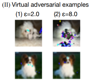
In VAT, we add small amounts of adversarial noise to images, then penalise our model for making different predictions on these images compared to the original images (source)

What is it?

VAT is inspired by the idea of adversarial examples. It has been shown that, if we peer inside an image classifier, we can exploit it and make it misclassify an image by just making tiny changes to that image.

In VAT, we try to generate such adversarial examples on-the-fly during training, and then update our network by saying that its prediction should not change in response to such small changes.

To do this, we need to first find the adversarial direction: the direction we should move our image \( X \) towards such that the model’s prediction changes as much as possible.

To find the adversarial direction, we:

1. Initliase a random-normal tensor \( \mathbf{r} \) with the same shape as \( X \).

2. Calculate the gradient of \( \mathbf{r} \) with respect to \( KL(f(X), f(X + \mathbf{r})) \), where \( KL(f(\cdot), g(\cdot)) \) is the Kullback-Liebler divergence between two probability distribution functions \( g(\cdot)) \) and \( g(\cdot)) \).

3. The normalised direction of this gradient is our adversarial direction, which we call \( \mathbf{d} \).

Once we have \( \mathbf{d} \), we move \( X \) in that direction by some small scaling factor \( \epsilon \). We then add a term to our loss that penalises the difference in the model’s predictions, i.e.:

\[loss_{\text{unsupervised}}(X) = KL ( f(X), f(X + \epsilon * \mathbf{r}) ) \\ loss = loss_{\text{supervised}}(X, y) + loss_{\text{unsupervised}}(X)\]

Since this \( loss_{\text{unsupervised}} \) term does not depend on any label \( y \), we can also use it with our unlabeled data

Implementation for FAT2019

There is a great Pytorch implementation of VAT on github. With this implementation, adding VAT to a model is simple:

vat_loss = VATLoss(xi=10.0, eps=1.0, ip=1)
# ... in training loop ...
lds = vat_loss(model, data)
output = model(data)
loss = cross_entropy(output, target) + args.alpha * lds

To use this repo for FAT2019 however, I needed to make a couple of changes to the implementation. The main problem is that it expects a classification model, so it uses softmax before the KL divergence over the classification distribution.

In our case, we use binary cross-entropy to predict a separate distribution for each label, rather than a distribution over labels. To overcome this I replaced the softmax with a sigmoid (where needed), and replaced the KL-divergence loss between the new and old predictions with the binary cross-entropy loss. For details, see the diffs between the Pytorch VAT repo and my fork.

Mean teacher

Mean teacher held the previous state of the art for SSL on CIFAR10 and other datasets, before being beaten by Mixmatch (which I descibe below). It is relatively simple to implement. Unfortunately though it seemed to produce little or no benefit for me in the competition.

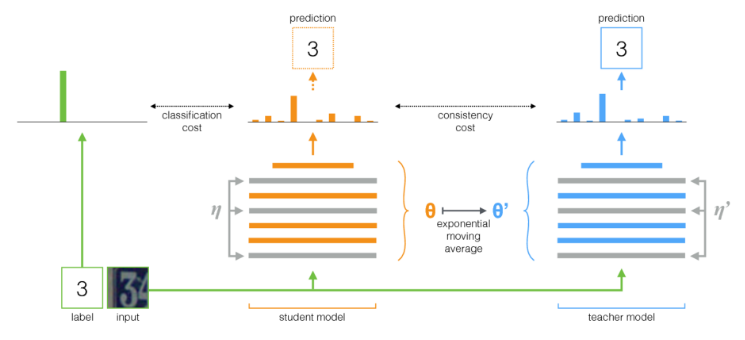
An overview of the mean teacher approach to SSL. A student model learns on a combination of a labeled dataset, and the predictions made by an exponential moving average of its history (the teacher model) (source)

What is it?

In semi-supervised mean teacher:

• We keep two copies of our model - a student model, and a teacher model
• Every K iterations (usually every epoch), we update our teacher model’s weights as an exponentially moving average (EMA) of the student model’s weights
• The student model is trained as usual on the labeled data, but in addition:
• We predict labels of our unlabeled data (plus random augmentation) using the teacher model. We then our student model for making different predictions on these same images (but with different random augmentation) to those predictions made by the teacher model.

Implementation for FAT2019

# We need to make a copy of our model to be the teacher
ema_model = Classifier(num_classes=num_classes).cuda()

# This function updates the teacher model with the student
def update_ema_variables(model, ema_model, alpha, global_step):
    # Use the true average until the exponential average is more correct
    alpha = min(1 - 1 / (global_step + 1), alpha)
    for ema_param, param in zip(ema_model.parameters(), model.parameters()):
        ema_param.data.mul_(alpha).add_(1 - alpha, param.data)

# ... in training loop
for epoch in range(num_epochs)
    # Update the teacher model
    update_ema_variables(model, ema_model, alpha, global_step)

    # Predict unsupervised batch (with augmentation) with the teacher
    with torch.no_grad():
        ema_model.eval()
        teacher_pred = ema_model(unsup_data_aug1.cuda()
        # We use sigmoid rather than softmax, as this is a
        # multi-label tagging task, rather than classification
        unsup_targ = torch.sigmoid(teacher_pred).data)

    # Predict unsupervised batch (with different augmentation)
    # with the student and add error to the loss
    unsup_output = model(unsup_data_aug2.cuda())
    loss_unsup = unsup_criterion(unsup_output, unsup_targ)
    loss += loss_unsup * unsup_loss_weight

Mixup

Another technique I (and many other Kagglers) played around with was mixup. In basic mixup, we combine two images \( \mathbf{X}_1 \) and \( \mathbf{X}_2 \) with a factor \( \alpha \) to become a single image, \( \alpha \mathbf{X}_1 + (1 - \alpha) \mathbf{X}_2 \). We then train on these combined images with combined labels \( \alpha \mathbf{y}_1 + (1 - \alpha) \mathbf{y}_2 \). Though it seems strange to ‘combine’ images like this, this seems to have a regularisation effect on models, and leads to better generalisation and results in general.

Applying mixup to audio perhaps makes more sense, as it is quite natural to add pieces of audio together, at least in the frequency domain. In the spectral domain, I’m not sure if this is still so natural. Still, it was a popular technique in this technique that seemed to provide some performance boost.

Mixmatch

Mixmatch is an SSL technique from Google Research. It achieved relatively large gains in SSL performance on CIFAR10 and other benchmarks, beating already-impressive state-of-the-art performance of other techniques.

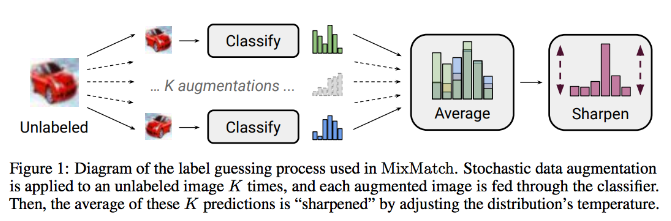
(Mixmatch produces labels for unlabeled data points by averaging their predictions over many augmentations, and then *sharpening this average prediction source)*

What is it?

In Mixmatch:

• We make K augmentations of a given unlabeled image, then predict it with our model to get K predictions
• We then average the K predictions to get a single prediction for that image
• We then sharpen this average prediction, such that confident classes become more confident, and unconfident classes become even less confident
• We then have labels for a batch of unlabeled data (plus our true labels for the batch of labeled data). We apply mixup over this whole set of labeled data, and train on it.

Implementation for FAT2019

One difficulty with transferring this method to FAT2019, was that the idea of sharpening predictions is not as well-defined in the binary cross-entropy case. Since, as mentioned above, this is in fact a ranking problem, our model could still perform very well, even if only outputting very low confidence predictions for all classes.

To sharpen in the binary cross-entropy setting, we essentially (either explicitly or implicitly) need to define some threshold at which we call a prediction ‘confident’, and increase its label in the sharpening, or ‘unconfident’, and decrease its label. A natural choice for this would be 0.5.

Ultimately though, I could not get Mixmatch to perform well, and I think this may be due to the fact that many predictions are quite low confidence in the final-trained models, even though they represent the most confident class. Perhaps selecting the most confident classes and sharpening them by setting their labels to 1 would be a better approach.

def sharpen(logit, T):
    return torch.sigmoid(T * logit)

def sharpened_guess(ub, model, K, T=0.5):
    with torch.no_grad():
        was_training = model.training
        model.eval()
        pr = torch.sigmoid(model(ub))  # shape = [B*K, 80]
        guess = pr.view(K, pr.shape[0] // K, -1).mean(0).data
        out = sharpen(guess, T).repeat([K, 1])
        if was_training:
            model.train()
        return out