Demystifying World Models: A Playable Diffusion Model

Building an interactive video diffusion model from scratch.

Playing our action-conditioned video diffusion model in real-time.

Background

“World Models” has become a bit of an overloaded buzzword lately. Depending on who you ask, it might refer to:

• Systems that reconstruct 3D environments from images or text prompts (e.g. World Labs’ Marble),
• Vision-Language-Action (VLA) models that take in visual feeds and output physical robotic control,
• Massive video foundation models that demonstrate an emergent intuitive physics of the world (e.g. Google’s Veo or OpenAI’s Sora), or
• Action-conditioned video generation models (e.g. DeepMind’s Genie series, Runway ML’s GWM Worlds).

This post focuses on that last category: treating video generation as an interactive simulator. Given recent frames and the player’s current control inputs, the network generates the next visual frames on the fly.

While systems like Genie or GWM Worlds rely on massive compute and proprietary datasets, the core mechanics behind them are surprisingly accessible.

In this post, we’ll build a minimal, playable proof-of-concept from scratch. We’ll cover:

• Data collection via a reinforcement learning (RL) agent that plays the game
• Designing and training a diffusion transformer that operates directly in pixel space
• Redesigning the temporal attention to use a causal KV cache to reach playable frame rates
• Fixing the autoregressive drift that causes long rollouts to degrade

On your marks…

Data Generation

To train a video generation model, you need a lot of videos. To train an action-conditioned video generation model, you also need actions that correspond to each video frame.

Example generated training data from CarRacing-v3.

To generate a large set of video-action data, I used Gymnasium. Its CarRacing-v3 environment is a top-down 2D car racing game with a randomly-generated track, continuous physics, and a simple action space:

\[\mathbf{a}_i = (\text{steer}, \text{gas}, \text{brake}) \in [-1, 1] \times [0, 1] \times [0, 1]\]

To generate episodes (packets of video frames + actions) of realistic gameplay, I used a pretrained reinforcement learning (RL) policy (vukpetar/ppo-CarRacing-v0-v3). Running gen_car_racing_data.py I obtained around 30 hours of $84 \times 96$ resolution, 25 fps RGB video, coupled with action data for each frame.

A Note on the Importance of Diverse Training Data

The RL agent was quite good at playing the game. But if the model only ever sees good driving, it won’t know what video frames to produce in response to things like driving off the track completely, or stopping. To get around this, I introduced variable levels of noise and smoothing to the RL model’s gameplay actions. As we will see later, this was probably insufficient, but for now, it was enough to move forward.

Action-Conditioned Video Generation with Diffusion

Diffusion models generate images by learning to iteratively reverse a gradual noising process. Once trained, a diffusion model can transform pure random noise into realistic images.

Diffusion models generate images by iteratively converting noise into new data samples (figure from DDPM).

Extending this to video is conceptually straightforward: we can just treat the video as a temporal sequence of frames and augment the architecture with temporal attention or 3D convolutions. I will assume readers are already familiar with the basics of diffusion and flow matching, and jump straight into the architecture.

Model Architecture: No VAE Required!

Contemporary video generation models (like Sora or Stable Video Diffusion) typically operate in the latent space of a pretrained Variational Autoencoder (VAE). Using a VAE reduces the dimensionality where we perform the computationally expensive diffusion process, making it crucial for high resolution video generation. In our case though, we’re dealing with just $84 \times 96$ pixels per frame, so we can comfortably skip the VAE and diffuse directly in pixel space.

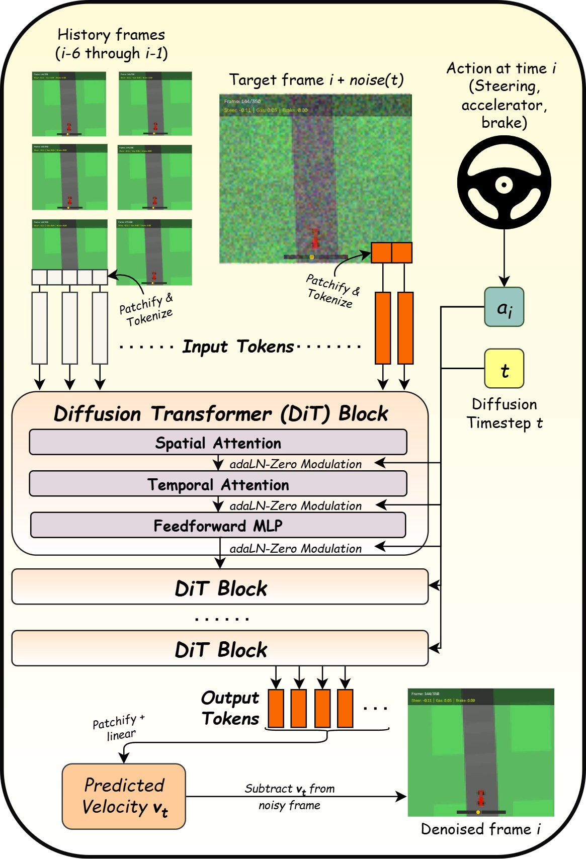
Even so, a $4 \times 4$ patch size yields $21 \times 24 = 504$ patches per frame. Over a 7-frame window (6 context + 1 target), that is $3{,}528$ spatiotemporal tokens. To support real-time interactive generation, we must avoid full spatiotemporal attention.

Enter factorised spatiotemporal attention – each DiT block consists of:

1. Spatial attention: tokens within each frame attend to each other.
2. Temporal attention: tokens at identical spatial locations across time attend to each other.
3. A standard feedforward MLP layer.

Our pixel-space DiT architecture with factorised spatiotemporal attention.

Conditioning on Actions & Historic Frames

As shown in the above figure, we supply the network with a history of 6 context frames (~240 ms at 25 fps). This window is long enough for the model to infer velocity, angular momentum, and track curvature trends, without paying excessive attention costs.

[Frame i-6] ... [Frame i-2] [Frame i-1] ──► [Frame i]
(---- 6 Clean Past Context Frames ----)     (Target Frame to Generate)

Besides historic visual context, the network also needs to know:

• The sequence of actions $\mathbf{a}_{i-6:i}$ (steering, gas, brake) accompanying both the context frames and the target frame,
• The diffusion/flow timestep $t$ currently being denoised.

To inject this information, we modulate each sublayer of our DiT blocks (spatial self-attention, temporal self-attention, and feed-forward MLP) using adaptive layer normalisation (AdaLN-Zero), driven by a per-frame conditioning vector.

In our case, conditioning works as follows:

1. Action embedding: Each 3D action $\mathbf{a}_j = (\text{steer}, \text{gas}, \text{brake})$ is projected via an MLP to $\mathbf{e}_{\text{action}, j}$.
2. Timestep embedding: The timestep $t$ is mapped via sinusoidal embeddings and an MLP to $\mathbf{e}_{\text{time}, j}$.
3. Summation: Both embeddings are summed into a single per-frame vector: \(\mathbf{c}_j = \mathbf{e}_{\text{time}, j} + \mathbf{e}_{\text{action}, j}\)
4. Timestep assignment:
   • Context frames use $t_j = 0$ (clean ground truth).
   • The target frame receives the sampled flow timestep $t \in [0, 1]$.

During training, we take a 7-frame slice (6 context frames + 1 target frame). The 6 context frames remain uncorrupted (diffusion timestep $t=0$), while the 7th frame undergoes the forward flow corruption process at a sampled diffusion timestep $t \in [0, 1]$. The loss is computed only on the predicted velocity of the target frame:

def forward_train_step(model, context_frames, target_frame, actions):
    """
    context_frames: (B, 6, C, H, W) - clean past frames
    target_frame:  (B, 1, C, H, W) - next ground-truth frame
    actions:       (B, 7, 3)       - action sequence across the window
    """
    b = target_frame.shape[0]
    t = torch.rand(b, device=target_frame.device)
    noise = torch.randn_like(target_frame)
    
    # Corrupt ONLY the target frame
    t_exp = t.view(b, 1, 1, 1, 1)
    target_noisy = (1.0 - t_exp) * target_frame + t_exp * noise
    target_velocity = noise - target_frame
    
    # Concatenate context (t=0) and target (sampled t)
    full_sequence = torch.cat([context_frames, target_noisy], dim=1)
    
    # Context frames get timestep 0; target gets sampled t
    timesteps = torch.zeros(b, 7, device=target_frame.device)
    timesteps[:, -1] = t
    
    # Predict velocity
    pred = model(full_sequence, timesteps, actions)
    loss = F.mse_loss(pred[:, -1:], target_velocity)
    return loss

Speeding Things Up: Causal Architecture + KV Caching

At this point, we have a working world model. But when we try to run it in real-time, we hit a roadblock: the forward pass is simply too slow. Even with just 4 Euler steps, we achieve just ~2 FPS on a 3060.

We can surely do better than 2 FPS! But how?

Notice that there is heavy redundancy during sampling: to generate just one frame with a 4-step Euler solver, we compute keys, queries, and values for the same 6 historic context frames four times in a row.

Then, when we slide forward to generate the next frame ($i+1$), 5 of those 6 context frames are still identical! We are effectively re-running the same attention computations over and over again.

Can we somehow cache the results of these repeated computations?

Causal Attention

In our original architecture, temporal attention was bidirectional: every frame could attend forward and backward across the window. But if frame $i$ attends to frame $i+1$, its representation changes whenever frame $i+1$ changes. The current frame changes at each new frame, and at every denoising step. This destroys any chance of reusing cached values in a bidirectional setup.

To unlock true real-time performance, we need to cache past representations. And to cache past representations in a transformer, the attention mechanism across time must be causal.

In bidirectional attention, past tokens' representations depend on future tokens, which makes caching impossible. In causal attention, tokens only 'look backwards'. This means older frames' Key ($\mathbf{K}$) and Value ($\mathbf{V}$) projections never change, so we can cache them!

Spatial self-attention within a frame remains fully bidirectional (a patch on the left of the car should obviously attend to a patch on the right of the car). But across time, information only flows from past to future.

The KV Cache in Action

Because temporal attention is now strictly causal, the Key ($\mathbf{K}$) and Value ($\mathbf{V}$) projections for all context frames depend only on the context frames themselves. They are completely independent of the noisy target frame being integrated.

This means we can compute the spatial features, keys, and values for the context frames exactly once, store them in a persistent circular buffer (the KV cache), and evaluate the model only on the single target frame during sampling.

The code snippet below illustrates how this works:

class CausalTemporalAttention(nn.Module):
    def __init__(self, dim):
        super().__init__()
        self.q_proj = nn.Linear(dim, dim)
        self.k_proj = nn.Linear(dim, dim)
        self.v_proj = nn.Linear(dim, dim)
        self.out_proj = nn.Linear(dim, dim)

    def forward(self, x, kv_cache=None):
        """
        x: (B, T, S, D) spatial tokens over time
            - Training: T > 1 (all frames in parallel, kv_cache=None)
            - Inference: T = 1 (just the current frame being denoised)
        kv_cache: optional tuple of (K_past, V_past),
                  each of which has shape (B, S, T_past, D)
        """
        B, T, S, D = x.shape  # During inference, T=1
        
        # Project to Q, K, V and permute to (B, S, T, D) to treat
        # each spatial position as an independent sequence over time.
        q = self.q_proj(x).permute(0, 2, 1, 3)
        k = self.k_proj(x).permute(0, 2, 1, 3)
        v = self.v_proj(x).permute(0, 2, 1, 3)

        # Inference: prepend cached keys/values from past context frames
        # (Note: During sampling, intermediate noisy states are not
        # added to the cache; the new frame is pushed only after all
        # denoising steps are complete).
        if kv_cache is not None:
            k_past, v_past = kv_cache
            k = torch.cat([k_past, k], dim=-2)  # (B, S, T_past + 1, D)
            v = torch.cat([v_past, v], dim=-2)  # (B, S, T_past + 1, D)
            
        new_kv_cache = (k, v)

        # Attention:
        # - Training (T > 1, no cache): apply causal mask
        # - Inference (T = 1, cached): Q is length 1 and attends
        #                              to all past + current KV
        out = F.scaled_dot_product_attention(
            q, k, v, is_causal=(T > 1 and kv_cache is None)
        )
        
        # Permute back to (B, T, S, D)
        out = out.permute(0, 2, 1, 3)
        return self.out_proj(out), new_kv_cache

As you can see, during inference:

1. Input x is just the single frame being denoised ($T = 1$).
2. Our kv_cache consists of Keys ($\mathbf{K}$) and Values ($\mathbf{V}$) previously computed for our 6 history frames.
3. Once denoising finishes, the new frame’s keys and values are appended to the rolling cache, evicting the oldest.

The result is an immediate $\sim 6$–$7\times$ speedup, enabling interactive frame rates.

The Exposure Bias Problem: Autoregressive Drift

With the causal architecture trained, it was now possible to play the model in real time.

While the model responded coherently to keypresses initially, after just a second of driving, the track distorted and the pixels dissolved into mush.

Conditioning on generated history, which the model was not trained on, causes the world model to break down after just a handful of frames.

This is a classic case of exposure bias (or autoregressive drift):

• During training: the model sees only pristine, ground-truth history.
• During inference: the model is conditioned on its own previous outputs, which contain imperfections and out-of-distribution pixel values.

Errors compound rapidly: a minor artifact in frame $i+1$ biases frame $i+2$, and within a few steps the inputs drift completely outside the training distribution.

The Fix: Context Noise Augmentation

How do we teach the model not to panic when fed imperfect context?

One principled approach is Diffusion Forcing (Chen et al., 2024), where every frame in the history is assigned an explicit, per-position noise level at both train and inference time. While powerful, implementing full diffusion forcing requires managing variable noise schedules across the KV cache at inference time.

Before going down that rabbit hole, I tried a much simpler hypothesis: what if we corrupt context frames during training with synthetic noise, but keep inference completely unchanged?

The corrupt_context Mechanism

During training, before passing the 6 context frames into the network, we independently corrupt each context frame with random noise. For each context frame $j \in \{i-6, \dots, i-1\}$:

\[\sigma_j \sim \mathcal{U}(0, \sigma_{\max})\] \[\tilde{\mathbf{x}}_j = (1 - \sigma_j) \mathbf{x}_j + \sigma_j \boldsymbol{\epsilon}_j, \quad \boldsymbol{\epsilon}_j \sim \mathcal{N}(\mathbf{0}, \mathbf{I})\]

Despite the frames now being noisy, during training, we still tell the model that the context frames are clean ($t = 0$) in the conditioning embedding.

def corrupt_context(context_frames, context_noise_max=0.2):
    """
    Corrupt context frames during training to build robustness
    against autoregressive exposure bias.
    
    context_frames: (B, T_ctx, C, H, W)
    """
    if context_noise_max <= 0.0:
        return context_frames

    B, T_ctx, C, H, W = context_frames.shape
    
    # Sample independent corruption intensity per context frame
    sigma = torch.rand(B, T_ctx, 1, 1, 1, device=context_frames.device) * context_noise_max
    noise = torch.randn_like(context_frames)
    
    # Apply flow-style corruption
    corrupted = (1.0 - sigma) * context_frames + sigma * noise
    return corrupted

This simple trick turned out to be surprisingly effective. Even though Gaussian noise doesn’t strictly match the artifacts our model produces during rollouts, it is apparently sufficient as a proxy for teaching the network to be robust to an imperfect history.

What’s Next?

We now have a working, playable, action-conditioned video world model that runs on a laptop GPU at around 8 FPS.

It works!

But there is still room for improvement. There are two main directions:

1. Improved Dataset Diversity. Our context noise fix solved autoregressive visual drift, but it cannot teach the model action sequences it has never witnessed. For instance, even without steering inputs, the car tends to steer correctly towards the track. This is because it was only trained on examples of already-good driving from our RL agent. The model does not know how to respond to poor steering, or even heavy braking. To fix this, we likely need a much more diverse training dataset. The authors of GameNGen got around this problem by training their RL agent from scratch, and recording episodes from all stages of the agent training.

2. Further Speedups. We hit 8 FPS with 4 Euler steps, but our model still requires a GPU to run, and the weights are around 450MB. Ideally, we would like to be able to run the model in a browser, with weights under 50MB. There are many possible avenues for speeding up the model, for instance:

   • Reflow / consistency models to distill the flow model down from 4 steps to a 1- or 2-step generator (using techniques like InstaFlow, Consistency Distillation, or Rectified Flow reflow)
   • Architectural changes, e.g., increasing patch sizes, adding a lightweight VAE, or distilling to a model with reduced width or depth
   • Quantisation: Compressing linear weights down to 16-bit or 8-bit. This alone could shrink the model from ~450MB to under 50MB and reduce memory bandwidth bottlenecks on integrated GPUs.

---

Thanks for reading! The training code and model checkpoint are available on GitHub here. Feel free to open an issue there or comment on the LinkedIn post if there is anything you would like to discuss!