In Raw Numpy: t-SNE

This is the first post in the In Raw Numpy series. This series is an attempt to provide readers (and myself) with an understanding of some of the most frequently-used machine learning methods by going through the math and intuition, and implementing it using just python and numpy.

You can find the full code accompanying this post here.

Dimensionality reduction

t-SNE is an algorithm that lets us to do dimensionality reduction. This means we can take some data that lives in a high-dimensional space (such as images, which usually consist of thousands of pixels), and visualise it in a lower-dimensional space. This is desirable, as humans are much better at understanding data when it is presented in a two- or three-dimensional space.

Take MNIST for example, a classic dataset of images of handwritten digits from 0 to 9. MNIST images are 28x28 pixels, meaning they live in 784-dimensional space. With t-SNE, we can reduce this to just two dimensions, and get a picture like this:

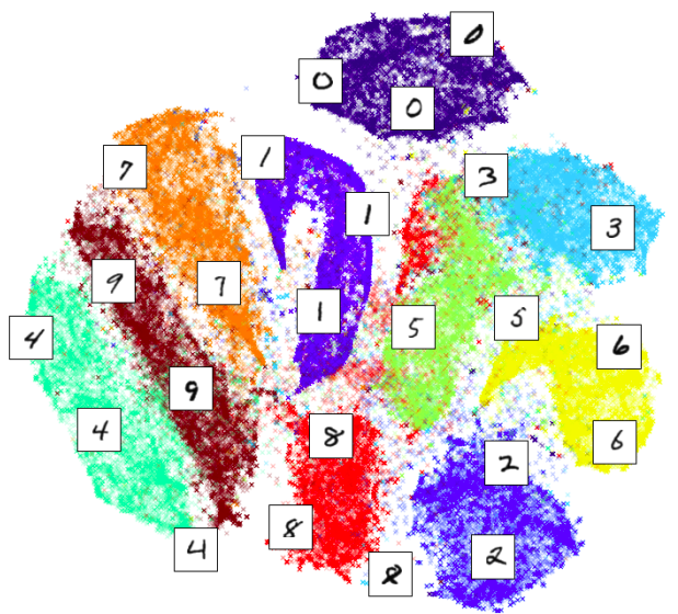MNIST images visualised in two dimesnions using t-SNE. Colours indicate the digit of each image. (via)

From here on, this article is focused on the implementation of t-SNE. If you want to understand more about dimensionality reduction in general, I recommend this great blog post from Chris Olah. If you’re interested in learning how to use t-SNE effectively, then definitely check this out.

Before t-SNE: SNE

t-distributed Stochastic Neighbor Embedding, or t-SNE, was developed by Geoffrey Hinton and Laurens van der Maaten. Their paper introducing t-SNE is very clear and easy to follow, and I more or less follow it in this post.

As suggested by the acronym, most of t-SNE is SNE, or the Stochastic Neighbor Embedding algorithm. We cover this first.

SNE: setup and overall goal

We have a dataset \(\mathbf{X}\), consisting of \(N\) data points. Each data point \(x_i\) has \(D\) dimensions. We wish to reduce this to \(d\) dimensions. Throughout this post we assume without loss of generality that \(d=2\).

SNE works by converting the euclidean distance between data points to conditional probabilities that represent similarities:

\[p_{j|i} = \frac{\exp \left ( - || x_i - x_j || ^2 \big / 2 \sigma_i^2 \right ) }{\sum_{k \neq i} \exp \left ( - || x_i - x_k || ^2 \big / 2 \sigma_i^2 \right )} \hspace{2em} (1)\]

Essentially this is saying that the probability of point \(x_j\) being a neighbour of point \(x_i\) is proportional to the distance between these two points (we’ll see where the \(\sigma_i\)’s come from a bit later).

One thing to note here is that we set \( p_{i|i} = 0 \) for all \(i\), as we are not interested in how much of a neighbour each point is with itself.

Let’s introduce matrix \(\mathbf{Y}\).

\(\mathbf{Y}\) is an \(N\)x\(2\) matrix that is our 2D representation of \(\mathbf{X}\).

Based on \(\mathbf{Y}\) we can construct distribution \(q\) as per our construction of \(p\) (but without the \(\sigma\)’s):

\[q_{j|i} = \frac{\exp \left ( - || y_i - y_j || ^2 \right ) }{\sum_{k \neq i} \exp \left ( - || y_i - y_k || ^2 \right ) }\]

Our overall goal is to pick the points in \(\mathbf{Y}\) such that this resulting conditional probability distribution \(q\) is similar to \(p\). This is achieved by minimising a cost: the KL-divergence between these two distributions. This is defined as follows:

\[C = \sum_i KL(P_i || Q_i) = \sum_i \sum_j p_{j|i} \log \frac {p_{j|i}} {q_{j|i}}\]

We want to minimise this cost. Since we’re going to use gradient descent, we’re only really interested in its gradient with respect to our 2D representation \(\mathbf{Y}\). But more on that later.

Euclidean distances matrix in numpy

Let’s code something. Both the formulas for \(p_{j|i}\) and \(q_{j|i}\) require the negative squared euclidean distance (this part: \(- || x_i - x_j || ^2 \)) between all pairs of points in a matrix.

In numpy we can implement this as:

def neg_squared_euc_dists(X):
    """Compute matrix containing negative squared euclidean
    distance for all pairs of points in input matrix X

    # Arguments:
        X: matrix of size NxD
    # Returns:
        NxN matrix D, with entry D_ij = negative squared
        euclidean distance between rows X_i and X_j
    """
    # Math? See https://stackoverflow.com/questions/37009647
    sum_X = np.sum(np.square(X), 1)
    D = np.add(np.add(-2 * np.dot(X, X.T), sum_X).T, sum_X)
    return -D

This function uses a bit of linear algebra magic for efficiency, but it returns an \(N\)x\(N\) matrix whose \((i,j)\)’th entry is the negative squared euclidean disance between inputs points \(x_i\) and \(x_j\).

As someone who uses neural networks a lot, when I see \( \exp(\cdot) \big / \sum \exp(\cdot) \) like in \((1)\), I think softmax. Here is the softmax function we will use:

def softmax(X, diag_zero=True):
    """Take softmax of each row of matrix X."""

    # Subtract max for numerical stability
    e_x = np.exp(X - np.max(X, axis=1).reshape([-1, 1]))

    # We usually want diagonal probailities to be 0.
    if diag_zero:
        np.fill_diagonal(e_x, 0.)

    # Add a tiny constant for stability of log we take later
    e_x = e_x + 1e-8  # numerical stability

    return e_x / e_x.sum(axis=1).reshape([-1, 1])

Note that we have taken care of the need for \( p_{i|i} = 0 \) by replacing the diagonal entries of the exponentiated negative distances matrix with zeros (using np.fill_diagonal).

Putting these two functions together we can make a function that gives us a matrix \(P\), whose \((i,j)\)’th entry is \( p_{j|i} \) as defined in \((1)\):

def calc_prob_matrix(distances, sigmas=None):
    """Convert a distances matrix to a matrix of probabilities."""
    if sigmas is not None:
        two_sig_sq = 2. * np.square(sigmas.reshape((-1, 1)))
        return softmax(distances / two_sig_sq)
    else:
        return softmax(distances)

Perplexed?

In the previous code snippet, the sigmas argument should be an \(N\)-length vector containing each of the \(\sigma_i\)’s. How do we get these \(\sigma_i\)’s? This is where perplexity comes into SNE. The perplexity of any of the rows of the conditional probabilities matrix \(P\) is defined as:

\[Perp(P_i) = 2^{H(P_i)}\]

Here \(H(P_i)\) is the Shannon entropy of \(P_i\) in bits:

\[H(P_i) = - \sum_j p_{j|i} \log_2 p_{j|i}\]

In SNE (and t-SNE) perplexity is a parameter that we set (usually between 5 and 50). We then set the \(\sigma_i\)’s such that for each row of \(P\), the perplexity of that row is equal to our desired perplexity – the parameter we set.

Let’s intuit about this for a moment. If a probability distribution has high entropy, it means that it is relatively flat – that is, the probabilities of most of the elements in the distribution are around the same.

Perplexity increases with entropy. Thus, if we desire higher perplexity, we want all of the \(p_{j|i}\) (for a given \(i\)) to be more similar to each other. In other words, we want the probability distribution \(P_i\) to be flatter. We can achieve this by increasing \(\sigma_i\) – this acts just like the temperature parameter sometimes used in the softmax function. The larger the \(\sigma_i\) we divide by, the closer the probability distribution gets to having all probabilities equal to just \(1/N\).

So, if we want higher perplexity it means we are going to set our \(\sigma_i\)’s to be larger, which will cause the conditional probability distributions to become flatter. This essentially increases the number of neighbours each point has (if we define \(x_i\) and \(x_j\) as neighbours if \(p_{j|i}\) is below a certain probability threshold). This is why you may hear people roughly equating the perplexity parameter to the number of neighbours we believe each point has.

Finding the \(\sigma_i\)’s

To ensure the perplexity of each row of \(P\), \(Perp(P_i)\), is equal to our desired perplexity, we simply perform a binary search over each \(\sigma_i\) until \(Perp(P_i)=\) our desired perplexity.

This is possible because perplexity \(Perp(P_i)\) is a monotonically increasing function of \(\sigma_i\).

Here’s a basic binary search function in python:

def binary_search(eval_fn, target, tol=1e-10, max_iter=10000, 
                  lower=1e-20, upper=1000.):
    """Perform a binary search over input values to eval_fn.
    
    # Arguments
        eval_fn: Function that we are optimising over.
        target: Target value we want the function to output.
        tol: Float, once our guess is this close to target, stop.
        max_iter: Integer, maximum num. iterations to search for.
        lower: Float, lower bound of search range.
        upper: Float, upper bound of search range.
    # Returns:
        Float, best input value to function found during search.
    """
    for i in range(max_iter):
        guess = (lower + upper) / 2.
        val = eval_fn(guess)
        if val > target:
            upper = guess
        else:
            lower = guess
        if np.abs(val - target) <= tol:
            break
    return guess

To find our \(\sigma_i\), we need to pass an eval_fn to this binary_search function that takes a given \(\sigma_i\) as its argument and returns the perplexity of \(P_i\) with that \(\sigma_i\).

The find_optimal_sigmas function below does exactly this to find all \(\sigma_i\)’s. It takes a matrix of negative euclidean distances and a target perplexity. For each row of the distances matrix, it performs a binary search over possible values of \(\sigma_i\) until finding that which results in the target perplexity. It then returns a numpy vector containing the optimal \(\sigma_i\)’s that were found.

def calc_perplexity(prob_matrix):
    """Calculate the perplexity of each row 
    of a matrix of probabilities."""
    entropy = -np.sum(prob_matrix * np.log2(prob_matrix), 1)
    perplexity = 2 ** entropy
    return perplexity


def perplexity(distances, sigmas):
    """Wrapper function for quick calculation of 
    perplexity over a distance matrix."""
    return calc_perplexity(calc_prob_matrix(distances, sigmas))


def find_optimal_sigmas(distances, target_perplexity):
    """For each row of distances matrix, find sigma that results
    in target perplexity for that role."""
    sigmas = [] 
    # For each row of the matrix (each point in our dataset)
    for i in range(distances.shape[0]):
        # Make fn that returns perplexity of this row given sigma
        eval_fn = lambda sigma: \
            perplexity(distances[i:i+1, :], np.array(sigma))
        # Binary search over sigmas to achieve target perplexity
        correct_sigma = binary_search(eval_fn, target_perplexity)
        # Append the resulting sigma to our output array
        sigmas.append(correct_sigma)
    return np.array(sigmas)

Actually… Let’s do Symmetric SNE

We now have everything we need to estimate SNE – we have \(q\) and \(p\). We could find a decent 2D representation \(\mathbf{Y}\) by descending the gradient of the cost \(C\) with respect to \(\mathbf{Y}\) until convergence.

Since the gradient of SNE is a little bit trickier to implement however, let’s instead use Symmetric SNE, which is also introduced in the t-SNE paper as an alternative that is “just as good.”

In Symmetric SNE, we minimise a KL divergence over the joint probability distributions with entries \(p_{ij}\) and \(q_{ij}\), as opposed to conditional probabilities \(p_{i|j}\) and \(q_{i|j}\). Defining a joint distribution, each \(q_{ij}\) is given by:

\[q_{ij} = \frac{\exp \left ( - || y_i - y_j || ^2 \right ) }{\sum_{k \neq l} \exp \left ( - || y_k - y_l || ^2 \right ) } \hspace{2em} (2)\]

This is just like the softmax we had before, except now the normalising term in the denominator is summed over the entire matrix, rather than just the current row.

To avoid problems related to outlier \(x\) points, rather than using an analogous distribution for \(p_{ij}\), we simply set \(p_{ij} = \frac{p_{i|j} + p_{j|i}}{2N}\).

We can easily obtain these newly-defined joint \(p\) and \(q\) distributions in python:

• the joint \(p\) is just \( \frac {P + P^T} {2N } \), where \(P\) is the conditional probabilities matrix with \((i,j)\)’th entry \(p_{j|i}\)
• to estimate the joint \(q\) we can calculate the negative squared euclidian distances matrix from \(\mathbf{Y}\), exponentiate it, then divide all entries by the total sum.

def q_joint(Y):
    """Given low-dimensional representations Y, compute
    matrix of joint probabilities with entries q_ij."""
    # Get the distances from every point to every other
    distances = neg_squared_euc_dists(Y)
    # Take the elementwise exponent
    exp_distances = np.exp(distances)
    # Fill diagonal with zeroes so q_ii = 0
    np.fill_diagonal(exp_distances, 0.)
    # Divide by the sum of the entire exponentiated matrix
    return exp_distances / np.sum(exp_distances), None


def p_conditional_to_joint(P):
    """Given conditional probabilities matrix P, return
    approximation of joint distribution probabilities."""
    return (P + P.T) / (2. * P.shape[0])

Let’s also define a p_joint function that takes our data matrix \(\textbf{X}\) and returns the matrix of joint probabilities \(P\), estimating the required \(\sigma_i\)’s and conditional probabilities matrix along the way:

def p_joint(X, target_perplexity):
    """Given a data matrix X, gives joint probabilities matrix.

    # Arguments
        X: Input data matrix.
    # Returns:
        P: Matrix with entries p_ij = joint probabilities.
    """
    # Get the negative euclidian distances matrix for our data
    distances = neg_squared_euc_dists(X)
    # Find optimal sigma for each row of this distances matrix
    sigmas = find_optimal_sigmas(distances, target_perplexity)
    # Calculate the probabilities based on these optimal sigmas
    p_conditional = calc_prob_matrix(distances, sigmas)
    # Go from conditional to joint probabilities matrix
    P = p_conditional_to_joint(p_conditional)
    return P

So we have our joint distributions \(p\) and \(q\). If we calculate these, then we can use the following gradient to update the \(i\)’th row of our low-dimensional representation \(\mathbf{Y}\):

\[\frac{\partial C}{\partial y_i} = 4 \sum_j (p_{ij} - q_{ij}) (y_i - y_j)\]

In python, we can use the following function to estimate this gradient, given the joint probability matrices P and Q, and the current lower-dimensional representations Y.

def symmetric_sne_grad(P, Q, Y, _):
    """Estimate the gradient of the cost with respect to Y"""
    pq_diff = P - Q  # NxN matrix
    pq_expanded = np.expand_dims(pq_diff, 2)  #NxNx1
    y_diffs = np.expand_dims(Y, 1) - np.expand_dims(Y, 0)  #NxNx2
    grad = 4. * (pq_expanded * y_diffs).sum(1)  #Nx2
    return grad

To vectorise things, there is a bit of np.expand_dims trickery here. You’ll just have to trust me that grad is an \(N\)x\(2\) matrix whose \(i\)’th row is \(\frac{\partial C}{\partial y_i}\) (or you can check it yourself).

Once we have the gradients, as we are doing gradient descent, we update \(y_i\) through the following update equation:

\[y_i^{t} = y_i^{t-1} - \eta \frac{\partial C}{\partial y_i}\]

Estimating Symmetric SNE

So now we have everything we need to estimate Symmetric SNE.

This training loop function will perform gradient descent:

def estimate_sne(X, y, P, rng, num_iters, q_fn, grad_fn, learning_rate,
                 momentum, plot):
    """Estimates a SNE model.

    # Arguments
        X: Input data matrix.
        y: Class labels for that matrix.
        P: Matrix of joint probabilities.
        rng: np.random.RandomState().
        num_iters: Iterations to train for.
        q_fn: Function that takes Y and gives Q prob matrix.
        plot: How many times to plot during training.
    # Returns:
        Y: Matrix, low-dimensional representation of X.
    """

    # Initialise our 2D representation
    Y = rng.normal(0., 0.0001, [X.shape[0], 2])

    # Initialise past values (used for momentum)
    if momentum:
        Y_m2 = Y.copy()
        Y_m1 = Y.copy()

    # Start gradient descent loop
    for i in range(num_iters):

        # Get Q and distances (distances only used for t-SNE)
        Q, distances = q_fn(Y)
        # Estimate gradients with respect to Y
        grads = grad_fn(P, Q, Y, distances)

        # Update Y
        Y = Y - learning_rate * grads
        if momentum:  # Add momentum
            Y += momentum * (Y_m1 - Y_m2)
            # Update previous Y's for momentum
            Y_m2 = Y_m1.copy()
            Y_m1 = Y.copy()

        # Plot sometimes
        if plot and i % (num_iters / plot) == 0:
            categorical_scatter_2d(Y, y, alpha=1.0, ms=6,
                                   show=True, figsize=(9, 6))

    return Y

To keep things simple, we will fit Symmetric SNE to the first 200 0’s, 1’s and 8’s from MNIST. Here is a main() function to do so:

# Set global parameters
NUM_POINTS = 200            # Number of samples from MNIST
CLASSES_TO_USE = [0, 1, 8]  # MNIST classes to use
PERPLEXITY = 20
SEED = 1                    # Random seed
MOMENTUM = 0.9
LEARNING_RATE = 10.
NUM_ITERS = 500             # Num iterations to train for
TSNE = False                # If False, Symmetric SNE
NUM_PLOTS = 5               # Num. times to plot in training


def main():
    # numpy RandomState for reproducibility
    rng = np.random.RandomState(SEED)

    # Load the first NUM_POINTS 0's, 1's and 8's from MNIST
    X, y = load_mnist('datasets/',
                      digits_to_keep=CLASSES_TO_USE,
                      N=NUM_POINTS)

    # Obtain matrix of joint probabilities p_ij
    P = p_joint(X, PERPLEXITY)

    # Fit SNE or t-SNE
    Y = estimate_sne(X, y, P, rng,
             num_iters=NUM_ITERS,
             q_fn=q_tsne if TSNE else q_joint,
             grad_fn=tsne_grad if TSNE else symmetric_sne_grad,
             learning_rate=LEARNING_RATE,
             momentum=MOMENTUM,
             plot=NUM_PLOTS)

You can find the load_mnist function in the repo, which will prepare the dataset as specified.

Symmetric SNE results

Here’s what the results look like after running Symmetric SNE for 500 iterations:

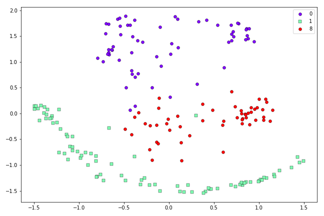Resulting two-dimensional representation of the first 200 0’s, 1’s and 8’s in the MNIST dataset, obtained via Symmetric SNE.

So we can see in this case Symmetric SNE is still quite capable of separating out the three different types of data that we have in our dataset.

Putting the t in t-SNE

Foei! That was a lot of effort. Fortunately to go from Symmetric SNE to t-SNE is simple. The only real difference is how we define the joint probability distribution matrix \(Q\), which has entries \(q_{ij}\). In t-SNE, this changes from \((2)\) to the following:

\[q_{ij} = \frac{ \left ( 1 + || y_i - y_j || ^2 \right ) ^ {-1} }{\sum_{k \neq l} \left ( 1 + || y_k - y_l || ^2 \right ) ^ {-1} } \hspace{2em} (3)\]

This is derived by assuming the \(q_{ij}\) follow a Student t-distribution with one degree of freedom. Van der Maaten and Hinton note that this has the nice property that the numerator approaches an inverse square law for large distances in the low-dimensional space. Essentially, this means the algorithm is almost invariant to the general scale of the low-dimensional mapping. Thus the optimisation works in the same way for points that are very far apart as it does for points that are closer together.

This addresses the so-called ‘crowding problem:’ when we try to represent a high-dimensional dataset in two or three dimensions, it becomes difficult to separate nearby data points from moderately-far-apart data points – everything becomes crowded together, and this prevents the natural clusters in the dataset from becoming separated.

We can implement this new \(q_{ij}\) in python as follows:

def q_tsne(Y):
    """t-SNE: Given low-dimensional representations Y, compute
    matrix of joint probabilities with entries q_ij."""
    distances = neg_squared_euc_dists(Y)
    inv_distances = np.power(1. - distances, -1)
    np.fill_diagonal(inv_distances, 0.)
    return inv_distances / np.sum(inv_distances), inv_distances

Note that we used 1. - distances instead of 1. + distances as our distance function returns negative distances.

The only thing left to do now is to re-estimate the gradient of the cost with respect to \(\mathbf{Y}\). This gradient dervied in the t-SNE paper as:

\[\frac{\partial C}{\partial y_i} = 4 \sum_j (p_{ij} - q_{ij}) (y_i - y_j) \left ( 1 + || y_i - y_j || ^2 \right ) ^ {-1}\]

Basically, we have just multiplied the Symmetric SNE gradient by the inv_distances matrix we obtained halfway through the q_tsne function shown just above (this is why we also returned this matrix).

We can easily implement this by just extending our earlier Symmetric SNE gradient function:

def tsne_grad(P, Q, Y, inv_distances):
    """Estimate the gradient of t-SNE cost with respect to Y."""
    pq_diff = P - Q
    pq_expanded = np.expand_dims(pq_diff, 2)
    y_diffs = np.expand_dims(Y, 1) - np.expand_dims(Y, 0)

    # Expand our inv_distances matrix so can multiply by y_diffs
    distances_expanded = np.expand_dims(inv_distances, 2)

    # Multiply this by inverse distances matrix
    y_diffs_wt = y_diffs * distances_expanded

    # Multiply then sum over j's
    grad = 4. * (pq_expanded * y_diffs_wt).sum(1)
    return grad

Estimating t-SNE

We saw in the call to estimate_sne in our main() function above that these two functions (q_tsne and tsne_grad) will be automatically passed to the training loop if TSNE = True. Hence we just need to set this flag if we want TSNE instead of Symmetric SNE. Easy!

Setting this flag and running main() gives the following 2D representation:

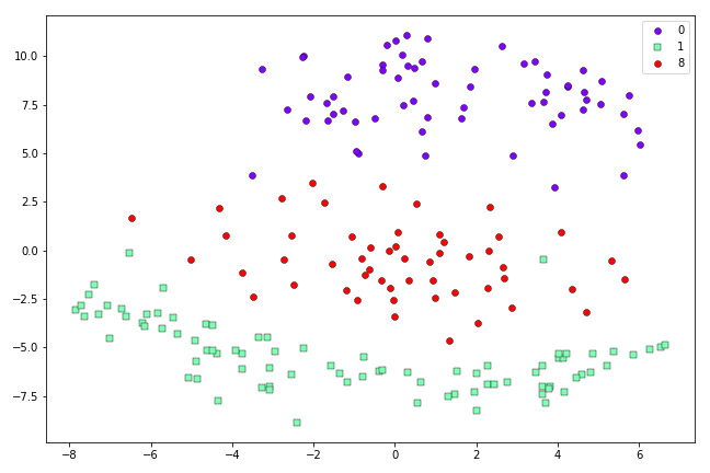t-SNE representation of the first 200 0’s, 1’s and 8’s in the MNIST dataset after 500 iterations.

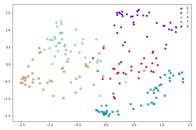
This looks a little better than the Symmetric SNE result above. When we scale up to more challenging cases, the advantages of t-SNE are clearer. Here are the results from Symmetric SNE versus t-SNE when we use the first 500 0’s, 1’s, 4’s, 7’s and 8’s from the MNIST dataset:

Symmetric SNE representation of the first 500 0’s, 1’s, 4’s, 7’s and 8’s in the MNIST dataset after 500 iterations.

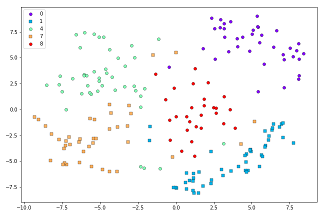t-SNE representation of the first 500 0’s, 1’s, 4’s, 7’s and 8’s in the MNIST dataset after 500 iterations.

It looks like the Symmetric SNE has had a harder time disentagling the classes than t-SNE, in this case.

Final thoughts

Overall, the results look a tad lacklustre as, for simplicity, I’ve omitted a number of optimisation details from the original t-SNE paper (plus I used only 500 data points and barely tuned the hyperparameters).

Still, this exercise really helped me to properly understand how t-SNE works. I hope it had a similar effect for you.

Thanks for reading!